SigmaPlot is now bundled with SigmaStat as an easy-to-use package for complete graphing and data analysis. The statistical functionality was designed with the non-statistician user in mind. This wizard-based statistical software package guides users through every step and performs powerful statistical analysis without having to be a statistical expert. Each statistical analysis has certain assumptions that have to met by a data set. If underlying assumptions are not met, you may be given inaccurate or inappropriate results without knowing it. However, SigmaPlot will check if your data set meets test criteria and if not, it will suggest what test to run.
| Describe Data
Single Group
Compare Two Groups
Compare Many Groups
- One Way ANOVA
- Two Way ANOVA
- Three Way ANOVA
- ANOVA on Ranks
Before and After
- Paired t-test
- Signed Rank Test
Repeated Measures
- One Way Repeated Measures ANOVA
- Two Way Repeated Measures ANOVA
- Repeated Measures ANOVA on Ranks
|
Rates and Proportions
- z-test
- Chi-Square
- Fisher Exact Test
- McNemars's Test
- Relative Risk
- Odds Ratio
Regression
- Linear
- Multiple Logistic
- Multiple Linear
- Polynomial
- Stepwise
- Best Subsets
- Regression Wizard
- Deming *
Correlation
- Pearson Product Moment
- Spearman Rank Order
Survival
- Kaplan-Meier
- Cox Regresssion
|
|
* = New Feature added in SigmaPlot
New Statistics Macros
- Normal distribution comparison with graph and statistics for preliminary quality control analysis. *
- Parallel line analysis to determine if linear regression slopes and intercepts are different. *
- Bland-Altman graph and statistics for method comparison.
Enhancements to Existing Features
- More accurate statistical errors in nonlinear regression reports for fit models with equality constraints. *
- P-values added for Dunnett’s and Duncan’s multiple comparison procedures. *
- Improved accuracy in multiple comparison statistics for higher-order effects in 3-Way ANOVA reports.
Enhancements to Existing Features
One-Sample Signed Rank Test
The One-Sample Signed Rank Test tests the hypothesis that the median of a population equals a specified value.
Feature Description – The one-sample t-test offered in SigmaPlot uses a single group of sampled data to test the null hypothesis that the mean of a population has a specified value. The value of the hypothesized mean is specified in the Test Options dialog.
One application of this test is the paired t-test, the simplest design for repeated measures. In performing a paired t-test, the difference between the measurements of the two groups is computed for each subject. These differences form a single group which is analyzed with a one-sample t-test to see if they are sampled from a population with zero mean.
The only assumption made in using the one-sample t-test is that the sampled population has a normal distribution. Although this test is known to be quite robust, it can still lead to misleading results if this assumption is not satisfied. This leads us to a non-parametric version of the one-sample t-test.
Computational Method - The idea is to provide a procedure, valid over a wide range of distributions, for testing a value that measures the central tendency of the population. For this purpose, the median of the population, rather than the mean, is the value we will test since it is more robust to sampling errors. Thus, using our sampled data, we want to test the null hypothesis that the median of a population is equal to some specified value. A rank-based test designed for this purpose is the (two-sided) Wilcoxon Signed Rank Test. We use a two-sample version this test now for our non-parametric paired t-test and a one-sample version can be implemented in a similar way. The basic assumption in using this test is that the underlying distribution of the population be symmetric about the median.
Calculations - Assume the null hypothesis is that the population median is M. If d(i) denotes the measurement for the ith subject, with n subjects total, then the algorithm proceeds as follows:
- Compute the differences: D(i) = d(i) – M.
- Ignore differences equal to zero and reduce n accordingly.
- Assign ranks to the absolute values of these differences in ascending order. If there are tied absolute differences, we apply the usual rule of assigning to each group of ties the average of the ranks that would have been assigned had the values been different.
- Let T- equal the sum of the ranks corresponding to the negative values of D(i), and let T+ equal the sum of the ranks corresponding to the positive values of D(i). Note that T+ + T- = n(n+1)/2.
- Put T = min(T-, T+).
- If T < Tα,n, where Tα,n is the critical value for the Wilcoxon distribution with significance level α, then reject the hypothesis that the population median is M. The basic idea is that if either rank sum is too small (and the other too large), then the lack of symmetry in the data about the value M is significant and the hypothesis should be rejected.
For values n>20, a normal approximation can be used to obtain the P-values. Including an adjustment for tied ranks, the parameters of this approximation are:
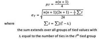
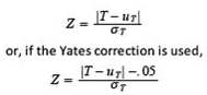
After computing the parameter, define in this formula, T can either be the sum of positive ranks or the sum of negative ranks, with identical results. After computing Z, its value is compared to the critical value Zα(2) of the standard normal distribution corresponding to the probability 1-α/2, where α is the significance level of the test. If Z> Zα(2), then we reject the null hypothesis that the population median is M.
In addition to the above hypothesis testing, we can compute a confidence interval for the median based on our data. One method is obtained by using the binomial distribution with probability (of success) p = .5. We first sort the original data in ascending order and then let d(i) be the ith smallest measurement, for i = 1 to n. Suppose we desire a 100(1-α)% confidence interval. We find the largest integer k such that
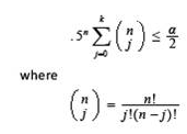
Then the lower limit of the confidence interval of the median is given by d(k+1) and the upper limit is given by d(n-k). Because of the discreteness of the binomial distribution, the confidence interval is typically a little larger than that specified.
There is also a normal approximation for the confidence interval for large sample sizes. In this case, the lower limit of the confidence interval is d(i) where i = [(n - Zα(2)n1/2)/2], where [∙] is the greatest integer operator and Zα(2) is defined as above. The upper confidence limit is given by d(n – i + 1).
For the implementation of the one-sample signed rank test, we will use the first method if the sample size is less than 100 and the second method otherwise.
Deming Regression
Deming Regression estimates the true linear relationship between two variables where the observations for both variables have measurement errors. A constant error value can be specified for each variable or a different error value can be assigned to each observation.
Example of Deming Regression Result Graph:
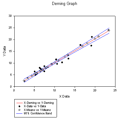
Feature Description – Deming Regression is a special case of Errors-In-Variables regression (also referred to as Type II Regression or the Random Regressor model). The problem is to determine the best straight-line fit to pairs of observations in which each coordinate has a measurement error from its true value. The computed slope and intercept values for the fit are estimates of the parameters values that define the line relating the true values of the two coordinates.
Certain assumptions are required to obtain a solution method for Deming Regression. The measurements for both coordinates are assumed to have a bivariate normal distribution with population standard deviations that have been specified (at least up to some constant multiple) by the user. All pairs of observations are assumed to be independently selected, and the two coordinates for each observation are also assumed to be independent. [top]
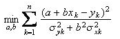
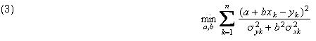
With the above assumptions, a maximum likelihood approach can be used to formulate the Deming Regression problem as an optimization problem. The input data for Deming Regression consists of pairs of observations, where the first coordinate refers to the independent variable and second coordinate refers to the dependent variable. Data errors for each variable, expressed as estimates of the standard deviations of the observations, must also be provided by the user. The main objective of Deming Regression is to determine the slope and intercept of the best-fit line. If the slope of the line is denoted by b and the intercept denoted by a, then maximizing the likelihood of obtaining the given observations is equivalent to the following minimization problem:
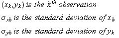
 Where, Where,
After solving this problem to obtain the equation of the regression line, we can compute estimates for the means of the normal distributions from which the observations of each coordinate were sampled. In addition to these estimates, other statistics will be provided in our reports for error estimation, confidence intervals and hypothesis testing. [top]
The above minimization problem is similar to the one used for ordinary linear least squares estimation where the measurement errors are only in the dependent variable. In fact, by setting the standard deviations of the independent variable to zero, we see that ordinary least squares estimation is a special case of Deming Regression. The appearance of the slope in the denominator greatly increases the difficulty in solving the minimization problem with the possibility of encountering more than one local minimum. Assuming the errors for each variable are not all zero, there is another important difference between Deming Regression and ordinary linear regression – you get the same regression line regardless of which variable is treated as the independent variable. This is not true for ordinary linear regression.
There are two types of Deming Regression based upon how the data errors are specified. When the data errors are constant among all measurements for each of the two variables, then we have a Simple Deming Regression problem. In this case, the minimization problem can be solved directly without an iterative technique. If the two constant error values for the independent and dependent variables are equal to each other, then Simple Deming Regression is often called Orthogonal Regression. In this case, the regression problem is equivalent to minimizing the sum of the perpendicular distances from the observations to the line. The other type of Deming Regression, General Deming Regression, allows arbitrary values for the error at each observation. The problem requires an iterative technique for its solution.
There are many ways to generalize Deming Regression that have been used in applications. There are versions where the model can be defined by a nonlinear or implicit relationship, or can contain more than one independent variable. The computer package ODRPACK95 has the capability to solve such problems. A multi-linear, constant errors version of Deming Regression can be solved by the techniques of Total Least Squares. There are also versions where the fit model is not a functional relationship between the true values of the observations, but a structural relationship between random variables.
Some Applications
1. Method Comparison Studies in Clinical Chemistry. The basic idea is to determine if there is a significant difference between the results of two measurement methods that are hypothesized to have the same scaling and zero bias.
2. Obtaining Isochron Plots in Geochronology. This is the universal method for dating rocks, sediments, and fossils. The plot is a straight line relating two isotope ratios found in several mineral samples from a common source.
3. Obtaining the linear relationship between turbidity and suspended solids used in water quality assessment.
Deming Model Assumptions - Suppose we are given N pairs of observations (x(k), y(k)), k = 1, …, N. For any random variable Z, let E(Z) denote its expected value. We make the following assumptions:
a. Each observation (x(k), y(k)) is the outcome of a random vector (X(k), Y(k)).
b. (X(k), Y(k)) has a bivariate normal distribution for each k.
c. The random vectors (X(k), Y(k)) are independent.
d. There exists numbers a and b such that expected values (or “true values”) of X(k) and Y(k) satisfy the condition:
E(Y(k)) = b*E(X(k)) + a , for all k
e. X(k) and Y(k) are uncorrelated for all k.
f. The standard deviations of distributions for X(k) and Y(k) are known for all k or are all known up to some common multiplier σ.
Given a set of observations and standard deviations for the input data, the primary goal of Deming Regression is to obtain estimates for the slope b and intercept a (also known as the structural parameters), estimates for the means or expected values E(X(k)), E(Y(k)) (also known as the nuisance parameters), and an estimate for the scaling factor σ. The estimates for the expected values E(X(k)), E(Y(k)) will be called the predicted or estimated means.
Optimization Problem - Using the above assumptions, the maximum likelihood function can be expressed as a product of bivariate normal density functions, one for each observation. We shall initially ignore the scaling factor σ for reasons to be explained later. Taking its logarithm (the log-likelihood function) and maximizing its value, subject to the constraints in part d., is equivalent to the following minimization problem:
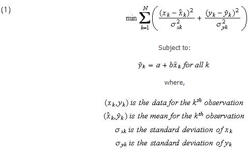
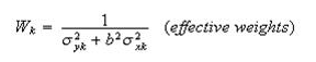
Recall that the unknown quantities in this problem are the means of the observations, the parameters a and b, and the scaling factor σ, which is implicitly included as a multiplier in each standard deviation. Using Lagrange multipliers, we can first minimize the sum of squares with respect to means, holding a and b fixed (this approach leads to what is sometimes called the concentrated likelihood function). After solving the equations obtained by setting the partial derivatives w/r to the means equal to zero, we obtain formulas for the estimated means in terms of the intercept and slope:
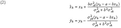
These equations are used to compute the values in the Predicted Means table of the report. Substitution of these equations into our sum of squares objective function (1) results in the new minimization problem:
To solve this minimization problem for the best-fit values of a and b, we take derivatives w/r to a and b and set the results to zero:
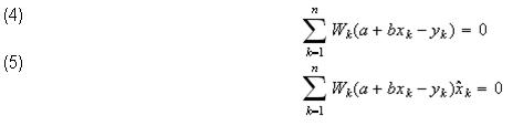
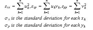
Where
Solving equation (4) for a, we have
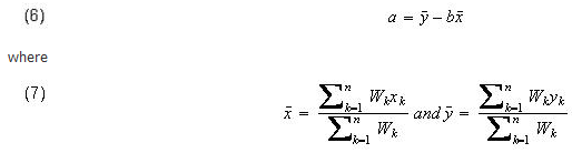
Using equation (6) to eliminate the parameter a, equation (5) can be rewritten as:
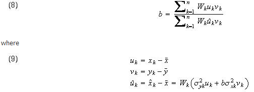
The solution for the best-fit parameters can now be found by solving equation (8) iteratively to find the slope, and then using equation (6) to find the intercept. Notice that if we solve (8) using the starting value b = 0, then the values of a and b after the first iteration are equal to the solution of the ordinary weighted linear least squares problem with errors only in the observations for Y.
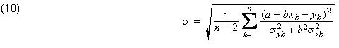
We have shown how one can obtain the best-fit parameters a and b, and we can then obtain the predicted means using equations (2). We could also have included the scale factor σ in our maximum likelihood function and obtained an estimate for it. The problem is that this estimate is inconsistent; that is it does not converge to the true value. A consistent estimate for σ, assuming the parameter estimates for a and b are also consistent, is given by:
The Case for Constant Data Errors - In Simple Deming Regression, the standard deviations for the measurements are constant for each of the variables X and Y. In this case, the values of the best-fit parameters can be obtained directly without the need of an iterative solution.
Referring to equation (8), we see that the effective weights cancel each other out in the numerator and the denominator when the data errors are constant for both X and Y. This equation can then rewritten as

Where
In solving this equation for b, we will have two solutions, but only one will lead to the minimum for (3):
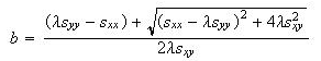
where

After solving for b, the value of a is obtained from equation (6).
Standard Errors of the Parameters - Based on Deming's work, York (1966, 1969) derived an exact equation for the straight-line, errors-in-both variables case with general weighting for the observations. In addition to correcting York's formulas for estimating error in the final parameters, Williamson (1966) simplified York's equation and eliminated the root-solving previously required. Williamson's method has been accepted as the standard in many fields for the least-squared fitting of straight-line data, errors in both variables.
Using the fact that both best-fit parameter estimates can be expressed as known functions of the observations, the estimates obtained by York and Williamson are based on the General Error Propagation Formula (Delta method).
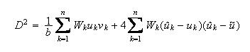
York and Williamson’s variance formulas for both the slope and intercept are given below. The standard errors for the parameters are obtained by taking square roots.
Using some notation defined in the previous section, let
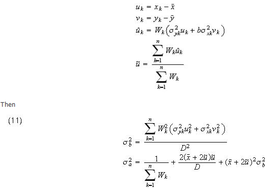
where
There is another estimation method for the standard errors that is based on the theory of maximum likelihood estimation, where the variance-covariance matrix is obtained as the inverse of the information matrix. For this approach, the variance of the slope and intercept are given below.
In addition to the notation defined above, let
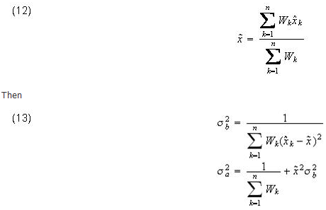
In general, these estimates give smaller values than those obtained by the York-Williamson method.
These are the formulas used to compute the parameter standard errors that appear in the report. If the user selects the option to interpret the supplied standard deviations for the data as only known up to a scaling factor, then that factor is estimated by formula (10) and the standard errors computed in the formulas above are multiplied by this factor to produce the standard errors in the report.
Covariance and Correlation of the Parameters - Using York’s method, the covariance and correlation of the parameters are given by:
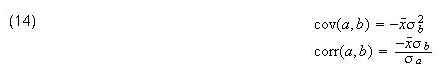
Using the MLE method, the covariance and correlation of the parameters (see formula 12) are given by:
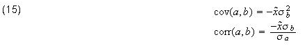
The covariance can be used to obtain standard errors and confidence intervals for simple functions of the parameters. The correlation measures the invariance of the linear relationship between a and b given by equation (6) as one resamples the data. For example, if the mean of x data is very small in absolute value, then the equation (6) shows the value of a depends little on the value of b and so the correlation will be close to zero. Also, if the standard error of b is small compared to the standard error of a, then our linear relationship is unlikely to remain the same after repeated resampling of the data since b will change very little compared to a change in a. In this case too, the correlation will be close to zero.
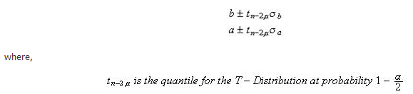
Confidence Intervals - Confidence intervals for the parameters are obtained the same way as in ordinary regression.
Suppose the user has selected 100(1-α)% confidence intervals (e.g. 95% confidence intervals imply α=.05). The confidence intervals for the slope and intercept are given by:
Vertical confidence bands for the regression line are computed as a series of confidence intervals for the means of Y at specified values of the independent variable X. To compute these, we need the variance of Y. Since the regression line is Y = bX + a, we have:

where each value on the right side can be computed from the formulas in the previous sections. At each value of X, our confidence band is given by:

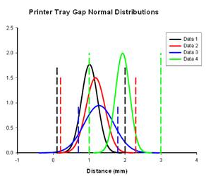
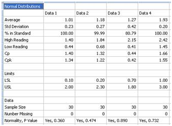
Normal Distribution Comparison
For a preliminary quality control analysis the engineer might collect data and quickly look at it assuming it is normally distributed. SigmaPlot generates normal distribution curves for each data set using the mean and standard deviation of the data. By examining the mean and variance (and other statistics) the engineer can quickly determine if a problem exists. The analysis in SigmaPlot produces a graph for visual interpretation and a report for numerical examination. The graph and report for printer tray gap measurements in the four tray corners is shown below. The normal distributions are compared to the limit lines also graphed and to each other. The data statistics are shown in the report.
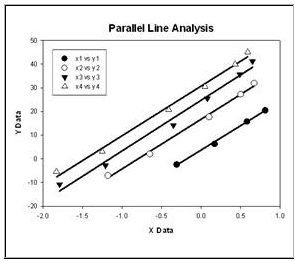
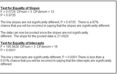
Parallel line analysis
Parallel line analysis determines if linear regression slopes and intercepts of multiple data sets are significantly different. It is commonly used in the biosciences to determine relative potency (EC50), bioassays for specific coagulation factors and inflammatory lymphokines and for radioimmunoassays for prostaglandins. In the example below the slopes are not different (P > 0.05) but the intercepts are (P < 0.0001). The report is written to describe the results in understandable language.
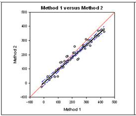
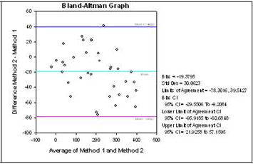
Bland-Altman method comparison technique
The Bland-Altman graph and statistics is another approach to method comparison. The Bland-Altman method is a plot that shows the difference between the two methods and computes the 95% limits of agreement. If the difference between the limits of agreement is small then the two methods agree and are considered to be the same. The graph on the left directly compares the results of measurements using both methods. The graph on the right plots the difference Y-X versus the mean (Y+X)/2 and uses the limits of agreement technique developed by Bland and Altman to determine if the two methods are the same.
References
- Cornbleet P.J., Gochman N., Incorrect least-squares regression coefficients in method-comparison analysis. Clinical Chemistry 1979, 25: 432-8
- Deming, W.E. 1943, Statistical Adjustment of Data, Wiley, New York. (Republished as a Dover reprint in 1964 and 1984, Dover, New York)
- Linnet K., Estimation of the linear relationship between the measurements of two methods with proportional errors, Stat Med, 1990; 9:1463-73.
- Linnet K., Performance of Deming regression analysis in case of misspecified analytical error ratio in method comparison studies, Clinical Chemistry 1998, 44:5, pp 1024-031.
- Martin, Robert F., General Deming Regression for Estimating Systematic Bias and Its Confidence Interval in Method-Comparison Studies. Clinical Chemistry 2000, 46: 100-4
- Press, W.H.; Teukolsky, S.A.; Vetterling, W.T.; Flannery, B.R. 1992, NUMERICAL RECIPES: The Art of Scientific Computing, Second ed., Cambridge Press, New York O'Neill, M; Sinclair, I,G.; Smith, F.J. 1969,
- Reed, B.C. 1992, Linear least-squares fits with errors in both coordinates. II: comments on parameter variances, Am. J. Phys., 60(1) pp 59-62
- Seber, G. A. F. and Wild, C. J. (1989) Nonlinear Regression, Chapter 10, New York: John Wiley & Sons.
- Williamson, J.H. 1969, Least-squares fitting of a straight line, Can. J. Phys., 46, pp 1845-1847
- York, D. 1966, Least-squares fitting of a straight line, Can. J. Phys., 44, pp 1079-1086
- York, D. and Evensen, Norman M. (2004), Unified equations for the slope, intercept, and statistical errors of the best straight line, Am. J. Phys., 72, pp 367-375
|