SigmaPlot provides seven different data smoothing algorithms that should satisfy most smoothing needs – negative exponential, loess, running average, running median, bisquare, inverse square and inverse distance. Each smoother contains options that make them very flexible. For example, unequally spaced data that occurs in clumps is better analyzed using the nearest neighbor rather than a fixed bandwidth method. Also, outlier rejection is available in some smoothers.
Two Dimensional Smoothing
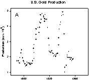
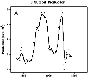
Smoothing is used to elicit trends from noisy data. The three examples in Tukey´s book Exploratory Data Analysis (Addison-Wesley, 1977) show the need for smoothing beautifully. The trends in the U.S. gold production from 1872 to 1956, Figure 1A, are fairly clear.
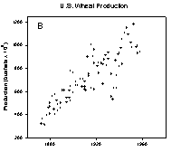
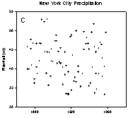
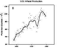
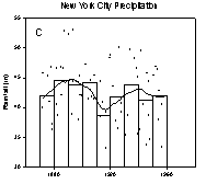
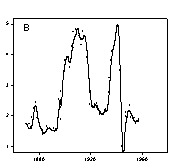
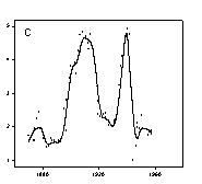
The peaks and valleys in the U.S. wheat production, Figure 1B, are less clear. I challenge you to visually find the trends in the annual New York City precipitation data shown in Figure 1C. The loess algorithm will be used to smooth these data sets. “loess” means locally weighted regression. Each point along the smooth curve is obtained from a regression of data points close to the curve point with the closest points more heavily weighted. The amount of smoothing, which affects the number of points in the regression is determined by the user. A weighted regression is performed for each point along the smooth curve.
Figure 1. Data with trends that are increasingly more difficult to visualize
loess smoothed curves for the three examples in Figure 1 are shown in Figure 2. The smoothed curves in Figure 2A and 2B make the trends in the gold and wheat data very clear. It is still difficult to visualize in the raw data the precipitation trend shown in Figure 2C. To confirm the results of the loess smoothed curve the histogram of average rainfall in ten year intervals was computed and superimposed on the smooth curve. There is a good comparison between the histogram and the loess smooth.
The loess smoothing parameters were varied to achieve the best visualization. A polynomial degree of one was used in all cases. A 0.1 sampling proportion was used in Figure 2A and B and 0.3 in Figure 2C. Since the data was unequally spaced along the x axis the nearest neighbor bandwidth method was used. The default number of intervals (100) for generation of the smooth curve was found to be the best. This generates a line using straight lines between curve points. Sometimes this leads to sharp corners in the smooth so the spline interpolation line type (Smoothed (spline)) was used.
Figure 2. Smoothed curves for data in Figure 1. A ten year average rainfall histogram is also shown in C.
Several of the smoothing methods, including loess, are based on local polynomial regression and the polynomial order is selectable. Increasing the order tends to include more high frequency components in the smooth. The effect of increasing the order from 1 (local linear regressions) to 2 (local quadratic regressions) is shown in Figure 3. The effect is to increase peak height magnitude and introduce additional high frequency components (wiggles) in B. A subsequent increase of the sampling proportion in C results in a smooth very much like the original for order 1 in A.
Figure 3. Effect of increasing the regression polynomial order. The order is 1 and sampling proportion is 0.1 in A. The order is increased to 2 in B and then the sampling proportion is increased to 0.2 in C.
Three Dimensional Smoothing
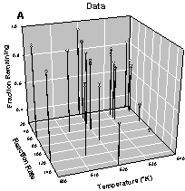
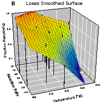
Visualizing spatial relationships in a three dimensional scatter plot can be very difficult. The strongest three dimensional cue is provided by an animated rotation of the data. Since this is not possible in paper publications we must resort to using drop lines, enclosing the graph with additional axes, etc. Figure 4 shows that a smooth surface also helps. This data describes the reaction characteristics on an isomer of hexane. The smooth surface B clearly shows the trends with respect to temperature and reaction rate whereas visualizing this in the scatterplot A is difficult.
Figure 4. The data trend in A is easily visualized with a loess smoothed surface, B.
This data is relatively sparse so a large sampling proportion 0.6 was required to avoid oscillations and spikes in the loess surface. A polynomial degree of 1 and the nearest neighbor bandwidth method were used. The Preview feature allows a quick comparison of smoothing methods on a given data set. For this data essentially equivalent smooth surfaces were obtained with the negative exponential and bisquare methods.
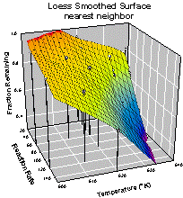
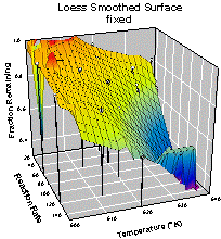
The bandwidth method option is also very useful. The nearest neighbor method works well for unequally spaced data. The data in Figure 3 is unequally spaced in both X and Y. Compare the smoothing results using the nearest neighbor and fixed methods shown in Figure 5. The result for the fixed method is about the best that could be obtained by varying the sampling proportion with a value of 0.8 shown.
Figure 5. Comparison of bandwidth methods for unequally spaced data. Nearest neighbor on the left and fixed on the right.
Additional Computational Details
Smoothers is a generic name for a variety of techniques that can be used to either smooth a data set by removing undesired high-frequency components (locations of rapid variation, such as noise contamination), or to resample dependent variable values to other independent variable locations using the values of the data at nearby points. The smoothing methods provided in SigmaPlot operate by weighting the data in a neighborhood of the smoothing location and applying linear or non-linear methods to combine the weighted values to produce a smoothed value. These non-parametric smoothing techniques provide a good complement to the parameterized curve/surface fitting facility (Regression Wizard) in SigmaPlot. For data subjected to measurement errors, noise, etc., either method can be used to predict behavior or to estimate true values.
The kernel used in the smoothing computation and the smoothing method are given in the following table.
Algorithm |
Weighting Kernel |
Method to Compute Smoothed Value |
Negative Exponential |
Gaussian |
Polynomial or Loess Fitting |
Loess |
Tricube |
Polynomial or Loess Fitting |
Running Average |
Uniform |
Mean |
Running Median |
Uniform |
Median |
Bisquare |
Biweight |
Polynomial Fitting |
Inverse Square |
Cauchy |
Mean |
Inverse Distance |
Inverse Distance |
Mean |
The equations used for each kernel are:
Kernel |
Kernel Formula (y=0 for 2D Smoothers) |
Uniform |
1 |
Biweight |
(1 - x2 – y2)2 |
Tricube |
(1 - sqrt(x2+y2)3)3 |
Gaussian |
exp(-x2-y2) |
Cauchy |
1/(1+x2+y2) |
Inverse Distance (3D only) |
1/sqrt(x2+y2) |